Parallelizing Nova - Visualizations and Mental Models behind Paranova

[krzhang]

(by Yan X Zhang and Aard Vark; this post is a copy of Parallelizing Nova - HackMD)

Suppose we wish to verify a sequence of computations of some iterated function F:
Z_0 \stackrel{F}{\rightarrow} Z_1 \stackrel{F}{\rightarrow} Z_2 \stackrel{F}{\rightarrow} \cdots where the i-th computation Z_i \stackrel{F}{\rightarrow} Z_{i+1} is an application of F to the previous computation’s output.

Technologies such as Nova IVC can be thought of as “folding compilers” – they take such a sequence of computations as input and outputs a “program” that uses the concept of folding to combine the computations into one that the verification could be deferred until the last step and only once on a “folded” computation. Our goal in this note is twofold:

1. to offer a beginner-friendly introduction to the main ideas, including a more compact visual language for folding computation.
2. to design a parallelization-friendly folding compiler parallelizing this folding process. Our presentation is heavily based on this document, but our scope is more minimalistic. We (collaboratively with the original authors) call this approach “Paranova.”

Visualizing Computation

First, we observed that conceptualizing Nova IVC and potential improvements can be confusing and people use very different mental pictures at different levels of abstraction. To disambiguate, we will try to separate these mental pictures at two levels, the computational level and the IWPC level.

Computation

First, we visualize computation. Broadly, computation is just ``work that needs to be verified.‘’ In our IVC setting (e.g. Nova or Paranova), a typical computation will represent the claim that, for some a \leq b, the calculation from z_{a} to z_{b} was performed correctly:
F(F(\cdots F(z_a))) = z_b. We’ll identify such a computation by the pair [a, b), which we can think of as the set \{a, a+1, \ldots, b-1\}, where the element i means “the i-th iterate of F was done correctly”: F(z_i) = z_{i+1}. As a base case, the notation [i,i+1) is just the singleton set containing computation i.

Now, we define folding (as in Nova) to be the act of combining 2 computations into one, so that verifying the resulting computation is (modulo cryptographic assumptions) verifying both computations.

1. For example, if we had an operation that folded, with our language above, [1, 4) and [4, 8) and also checks some consistency conditions (specifically, while F(z_3) = z_4 and F(z_4) = z_5 are part of the computations [1,4) and [4,8) respectively, checking that the z_4 from the first constraint equals the z_4 from the second constraint is not; we need to do that separately), then we have effectively turned the two computations into a single one equivalent to [1,8).
2. If we repeat this process, we would be able to turn the n verifications involved in checking F^{(n)}(z_0) = z_n into a single verification of the computation [0, n); if the saving of (n-1) verifications exceeds the overhead of folding, then this is an improvement.

Now, there is a catch to this. When we fold two computations, we don’t exactly get one computation; we get a folded computation but also another computation we need to verify later, which is the clam that the folding itself was done correctly. We summarize what we discussed so far in the following visual model of a single fold:

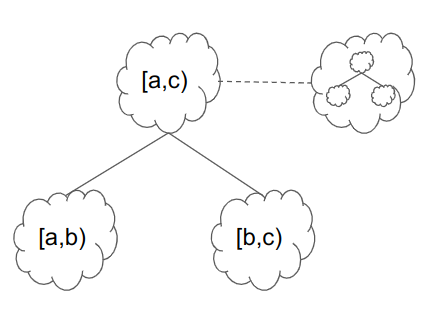
In this picture, the squigglys represent pieces of computation. We are folding computations [a,b) and [b,c), corresponding to steps \{a, a+1, \ldots, b-1\} and \{b, b+1, \ldots, c\} respectively in the original chain of applications of F. This means altogether they embed steps \{a, a+1, \ldots, c-1\}, or [a, c). The upper left new computation represents these steps.

However, by folding together 2 pieces of computation, we have actually created a new piece of computation we need to prove later: the act of folding itself! We denote this with the dashed line from the folded circle, pointing to a new squiggly (computation) that needs to be eventually verified in the scheme. More specifically, it consists of

• verifying that the R1CS in the two squares correctly folds to the R1CS in the new upper left computation;
• verifying that indeed b = b so the two computations “match” correctly
• verifying that the output of the [a,b) computation equals the input of the [b,c) computation.

This creates a couple of problems:

1. suppose we want to fold n computations [0,1), [1,2), … [n-1, n). First, we fold [0,1) and [1,2) to get [0,2). But then we also have this extra squiggly created for the folding. So if we were to fold everything, we’d get [0, n) as we hoped, but then we would end up with (n-1) extra squigglies, and we still have n pieces of total computation to fold. This way, we end up right where we started, all because every 2 pieces of computation fold into… 2 more pieces of computation, which does not seem to make progress.
2. Recall that the “types” of computation in the upper left and right squigglies are different. The upper left squiggly, like the original bottom two squigglies, correspond to (possibly nested) applications of F. However, the upper right squiggly checks folding and consistency between computations. This means that it is a different type of computation and might not fold nicely with the “evaluations of F” type of computation.

It turns out we can solve both of these problems at once! If we had a computational unit that treats different types of computation separately and can perform them at the same time, we would be able to actually compress the progress. This intuition will help us understand IWPCs, which we now introduce.

IWPC

For us, an IWPC (instance-witness-pair collection) is a collection of R1CS instance-witness pairs taking one of the following two types:

1. Base (in Nova, (u, w)): a circuit that represents the claim that some new computation or algorithm was carried out correctly. This may include some or all of:
   a. F-computation: the computation of a single iteration of the function F.
   b. Non-F computation: computation that verifies some folding, which would include the folding itself (including the computation of the hash function used for Fiat–Shamir randomness) and also consistency checks (for example, to verify that the output of one iteration of F agrees with the input of the next).
2. Folded (in Nova, (U, W)): a folded combination of instance-witness pairs from previous nodes. This combination represents the claim that some computations in previous nodes were done correctly.

The motivation of this notation comes from that of nodes from Paranova [^Paranova], which one can think of as a pair of IWPCs, one of the base type and one of the folded type. Paranova uses two types of nodes, base and intermediate, which roughly contain a base IWPC and a folded IWPC, respectively.

The idea of there being different types of computation inside the base computation is that we can skirt the “2-to-2 problem” by using this extra ``space’’ inside the node:

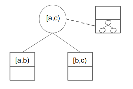
The entries in this picture are IWPCs now, not just computation. Furthermore:

1. squares are base IWPCs. The top half can contain F computation, and the bottom half can contain non-F computation (folding and consistency checks).
2. circles are folded IWPCs. So [a,b) and [b,c) would combine into [a,c), modulo the non-F folding and consistency checks which are needed. As before, we use dotted lines to point to a new set of non-F computations that need to be verified.

The main idea is that even though we still went from 2 vertices to 2 vertices, we are able to consistently add in a new computation (in the upper-right node’s [c,d) slot), so repeating this process actually makes forward progress! To see this, we can visualize a high-level sketch of Nova IVC with this picture:

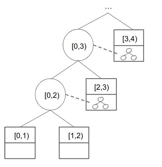
In this example, we start by folding the first two F computations [0,1) and [1,2) into a folded [0,2) and a new non-F computation to check (the [1, 2) \rightarrow [1,3) fold). However, the right (base) IWPC contains both this non-F computation and an additional F computation for [2,3). These two IWPCs can then be folded with the folded [0,2) to get [0,3) = \{0, 1, 2\}, etc., and we indeed are able to make incremental progress and fold everything into one node.

Fan-ins

Folding is typically done in a linear fashion: as a mostly accurate model, imagine the computation being represented by some matrix of numbers. Then most implementations of folding M_1 and M_2 comes down to creating a matrix sum M_1 + rM_2, where r is some random scalar. This means there is no theoretical obstacle to fold more than 2 IWPC’s at once (but for engineering reasons, especially accumulation of folding error terms, 4 seems to be the upper bound of what is currently feasible). We say that we have m-to-1 fan-in if we can fold m IWPC’s into one folded IWPC and, as before, creating an extra piece of non-F base computation to check later.

Question how do different fan-in options affect parallelizing Nova?

At least with current folding technologies, there is no theoretical obstacle to folding a mix of folded and base IWPCs. In practice, the different combinations might require different declarations and create some overhead. For example, a 3-to-1 fan-in that folds 2 base and 1 folded IWPC would look like this:

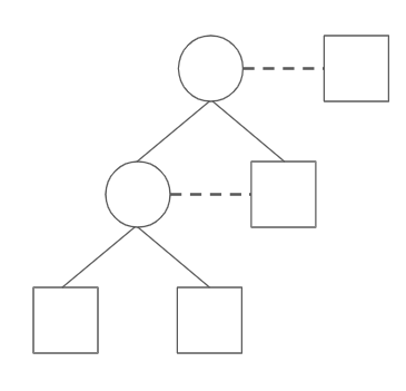
For the rest of this section (and article, when needed), we suppress the text and internal boundaries inside the squares to de-clutter the picture. To summarize as an abstract visualization game, having m-to-1 fan-in means that we can fold m circles and squares into one circle via solid edges and draw a dashed edge to a new square. Revisiting Nova IVC as using 2-to-1 fan-in, our simplified picture looks like this:

Now, we can imagine that if we were to have 3-to-1 fan-in, we would be able to generate something like this:

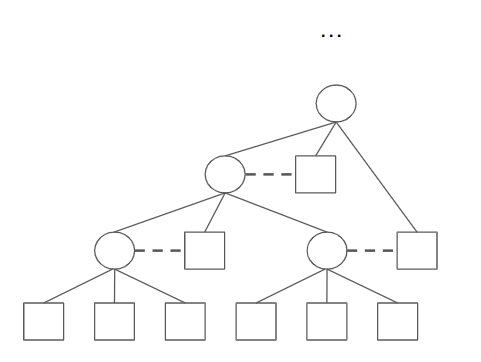
Which looks fairly ad-hoc. 4-to-1 is nice since the parity makes things work out nicely:

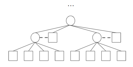
The main idea is that 2-to-1 (as in plain Nova) doesn’t allow for any nice tree structure - things pretty much still have to be done sequentially. However, once we have higher fan-in, we might be able to parallelize the work. In particular, the 4-to-1 fan-in seems perfect for making binary trees, so it is the current design in Paranova.

Elliptic Curve Pairs

There is one more source of complexity that will offer huge gains in efficiency. In the underlying cryptographic setup, we’re actually doing computations with points on an elliptic curve, using elliptic curve arithmetic, instead of numbers. This means, for example, that when we do a folding, we’re actually doing a bunch of computations on points of our elliptic curve.

When we fold, we create a new (non-F) computation that checks the folding. The key technical point is this: It’s hard for a node that does computations on an elliptic curve E to check a computation on the same curve E. It’s much easier if you work with a pair of elliptic curves. A pair is two elliptic curves E_1 and E_2, where a node working on E_1 can cheaply check computations on E_2, and a node working on E_2 can cheaply check computations on E_1.

We will not be able to cover all the basics of elliptic curve pairs, but we try to outline what we need here:

1. An elliptic curve E is the set of solutions (x, y) to a certain type of equation, where x and y lie in a finite field, called the ground field.
2. We say that E_1 and E_2 form a 2-cycle (pair) of curves when the number of points on E_1 is the size of the ground field of E_2, and vice-versa. Functionally, this means that a computation on E_1 can be verified in native arithmetic on E_2, and vice-versa.
3. In Paranova (and many other protocols in ZK), we assume we are given a pair of curves, in our case Pasta curves. We call one of them primary and one secondary.

This gives us two additional rules on our computation (and also our visualization):

1. Each IWPC is “on” either E_1 or E_2, meaning its computation is written over curve elements in the corresponding curve. (in the picture: we need the shapes to lie on two sides of some line, corresponding to the two curves)
2. When we fold two nodes, the newly created folding computation induced by the folding must lie in the other curve. (in the picture: each dashed line must cross over to the other side)

Remark: We don’t have to use an elliptic curve pair: we could work over a single elliptic curve E, and use a calculation on E to verify the folding on the same curve E. This is known as wrong-field arithmetic. Using an elliptic curve pair typically makes the IWPC 100-200x shorter than wrong-field arithmetic – a big enough saving that we typically consider elliptic curve pairs to be essential.

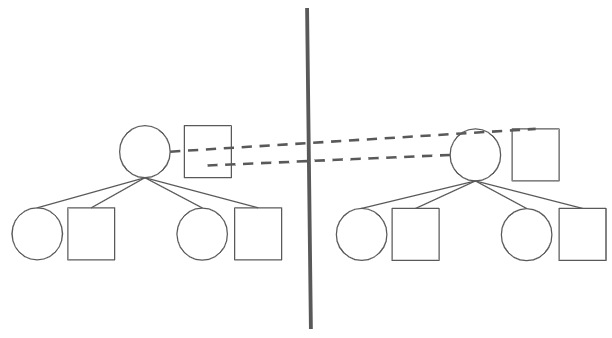
It would be nice to have some general process to take one of our pictures and turn it into a picture that obeys these rules. We introduce such a process that we call mirroring, which takes as input an unmirrored picture (such as any picture we have drawn so far about IWPCs that do not consider elliptic curves) and outputes a mirrored picture which obeys the two additional rules above:

1. Mirroring inputs a picture G with n vertices and will output a mirrored picture with 2n vertices.
2. Draw a vertical line down the middle of the picture: IPWCs drawn on the left side will be on the primary curve and those on the right will be on the secondary curve.
3. For vertices (IWPCs), create a copy of G's vertices on both sides.
4. For solid lines, have each copy contain the same solid lines as in G.
5. For a dashed line from a circle C to the square S, draw a dashed line from C to S's mirror image in the other curve instead. Note that this appears in pairs, once for C and once for its mirror image.

To see an example of this construction, we present the mirrored picture of Nova IVC:

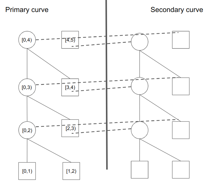
1. The individual computations all lie on the primary curve.
2. As in the previous visualization, we continuously extend a cumulative folded computation in the intermediate (circle) nodes in the primary curve.
3. However, we need a mirrored copy of “dummy” computations in the second curve. They do not actually verify computations; the primary reason they exist is that they encode the folding computation for nodes in the primary curve. (as an exercise to the reader, note that the bottom right two squares can be discarded safely)
4. After the initial two computations are folded, each additional base node (in our picture, [2,3) and up) also verifies a folding computation in the other curve.

Before going on, observe that since we have to effectively double the number of nodes in Nova IVC, we have a “2:1 waste”: if we have to fold n computations, we need around 2n nodes. Now, as a mental experiment, suppose half of our computations can be written in the other curve. This means all of the square boxes on both the left side (primary curve) and the right side (secondary curve) are are all doing useful computation. In this limit, there is no waste; our 2n nodes do 2n worth of computation.

Question: is mirroring our best construction? Are there optimizations we should worry about? How do we minimize the ``waste’’ from having 2 curves?

Paranova

We are now ready to present Paranova (heavily based on this document, with collaboration with original authors), which is a specific approach to parallelizing Nova. First, we define a node to be a pair of IWPCs, one base and one folded. For a node X, we use the lower case X.u to denote the base IWPC and capital X.U to denote the folded IWPC (this is like Nova, which uses (u,w) for instance-witness pairs and (U,W) for folded instance-witness pairs; we compress the notation into a single letter since the additional detail is unencessary). The main design of Paranova is that it is a binary tree of nodes, powered by a 4-to-1 fan-in that folds 2 base and 2 folded IWPCs.

To see this, consider a single fold. Each 4-to-1 fold folds 4 IWPCs, which we interpret as folding 2 nodes. Locally, we call the left node L, the right node R, and the folded node P (for parent). For each node X (where X \in \{L, R, P\}, we use For example, L.u would mean the base computation on the left child node.

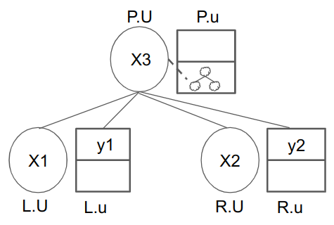
In the picture above, our strategy is to make sure that the contents of the 4 IWPCs (X_1, y_1, X_2, y_2), where each element could be some set of computations in [a,b) form, correctly union to the content X_3 of P.U. Per the Elliptic Curves section, we use our mirroring construction to produce a “true” mirrored picture with 8 IWPCs being folded:

What remains is to assign the work correctly to the squares. There are many different ways to do this. One intuitive way is the following:

1. As usual, have the squares on the left contain base computations.
2. Assume for simplicity that we have 2^n-1 computations 1 through 2^{n}-1. (for this example, we do not start at 0; the numbers work out a little better) Just use padding/dummy computations if we do not have exactly this number.
3. Draw a complete binary tree of nodes (on each curve). For the bottom row in the primary curve, have the squares contain all the odd computations 1, 3, … 2^{n}-1.
4. For any node P in a row in the primary curve except the bottom, it is easy to see inductively that its children contains cumulatively some computation sets [a, b) and [b+1, c) respectively. We assign its square the computation b = [b, b+1). Then, the subtree rooted at P would contain again a contiguous set of computations [a, c).
5. Inductively, it can be shown that the top node in the primary curve has the middle computation 2^{n-1}. In fact, the nodes correspond to a binary search tree; every node’s square contains the computation that is the median of all of its children.

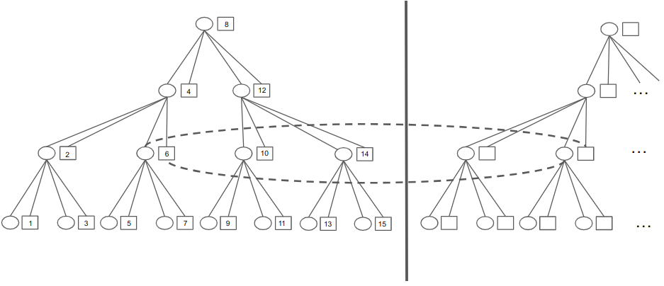
We visualize an example using 15 computations above. In the picture,

1. As stated, the circles on the left side (except the first row) should contain a contiguous set of computations except a single omission that is filled by the square it is next to. For example, the node with the square containing computation 4 has its circle contain the folding of computations [1,4) unioned with [5,8), so along with the 4 in its square, the node would account for the computation set [1, 8).
2. we suppressed the dashed lines as it would get very confusing; just recall that each circle above the last row has a dashed line to its square node-neighbor’s mirror image in the other curve. We have drawn a single pair of these dashed lines as an example.
3. there is much room for optimization. For example, if we have the flexibility of different types of 4-to-1 fan-ins, we can replace the bottommost row of circles with squares with content (right now they are just dummy “folded” computations). Also, as before, the last row on the secondary (right) curve is entirely unnecessary.

Update 6/22/23

The paper (new as of late June 2023) found a security bug in a recent implementation of Nova IVC on a cycle of two elliptic curves – roughly speaking, the verifier did not verify all the R1CS constraints that need to be verified on both curves. The paper gives a correct modification of two-curve Nova, along with a formal proof of security.

Acknowledgments

First and foremost, we thank the authors of Paranova [^Paranova] for a first design of these topics. We thank Nalin Bhardwaj, Carlos Pérez, Yi Sun, Jonathan Wang, and Lev Soukhanov for useful discussion. We thank 0xPARC for organizing the ZK Week in Zuzalu, where many of these discussions took place.